Risk and Ignorance, the way I understand it

There are limits to what we know, and a lot of the time we are trying to figure out ways in which to make outcomes insensitive to our ignorance. Risk avoidance in the daily sense, to me, is ignorance avoidance, the seeking of profitable action crafted to avoid areas of ignorance. My ignorance being special to me, by paying attention to it I make maximal use of my Richardian comparative advantage with respect to others.

I don't understand what others do or do not know very well, so I use the shortcut of estimating comparative advantage by virtue of my absolute level of certainty in the subject matter. Sometimes, however, I come across subjects which nobody really knows anything about. If others also maximize their comparative advantage by sticking to opportunities of high absolute certainty, then opportunities of low absolute certainty and high relative certainty would be one type of under-exploited opportunity I know to expect to find.

This, I feel, is the risk-tolerance of the entrepreneur. It is quite distinct from financial risk as we treated it two posts ago, which in fact is a rather strange animal because it is simultaneously uncertainty about the outcome and certainty about probabilities, an unlikely state in the real world.

I am guessing that the mind machinery for dealing with possibilities and future counterfactuals is more like Monte Carlo than anything else. We think of detailed alternate future paths and use those to weigh the value of an option - sounds like the algorithm a particular go-playing AI uses. What makes for a good Monte Carlo sampling strategy? How does one become a better Monte Carlo sampler? Answers to those would make for big advances in thinking.
2 comments
Carl

Chiao, I read this and your previous post on financial risk with great interest. Connecting the two posts, you could continue to say that risk takers are being compensated for more than only undiversifiable risk (ala CAPM), but are in fact being compensated for assymmetric ignorance. But of course, assymmetric ignorance probably implies inefficient markets, which probably is assumed by CAPM.

But even more of interest to me is another continuation of this discussion: I have been thinking, like you, about the decision process involved in seeking competitive advantage.

Often, in the course of seeking competitive advantage, we are faced with a seemingly simple situation: we must choose between two possibilities with outcomes sufficiently characterized by normally distributed random variables X and Y. I find usually, I can estimate both expected value and variance of these variables sufficiently for our purposes.

Let us say, for example, X has both a greater expected value and a greater variance than Y. Because of the variance, although X has higher expectation, perhaps Y should be chosen.

What confuses me is how to account for this variance. In another words, what is the risk discount? I do find the quadratic model perhaps insufficient for the practical needs of an entrepreneur.

Your thoughts?

Chiao

@Carl

Assuming a normal distribution and a general utility function is to a very large extent the same as assuming a quadratic utility function and a general distribution. (You can sort of see this from how adding any two quadratic functions gets you another quadratic function and multiplying any two gaussians gets you another gaussian.)

I don't think an entrepreneur should care about these crude strategic pictures. What they should really care about most, I think, are tactical issues, the thousand papercuts that grind at startups. For example, I think the variance in employees and co-founders completely overrides anything else (i.e. how they respond to seemingly impossible tasks). Shortly after you shatter all tactical issues, you'd be in the position to hire a proper CEO I think. :)

The twice-iterated prisoner's dilemna

Familiar with prisoner's dilemna? It's a game, played between two people, with two responses available to each side, making for a total of 4 possible outcomes. The context is that of two accomplices caught by the police, and the choice is to either stay silent or confess. Outcomes are as follows (from the wikipedia page):

B stays silent B confesses
A stays silent Each serves 6 months A serves 10 years
B goes free
A confesses B serves 10 years
A goes free
Each serves 5 years

What should one do as A? In this case it is easy to decide, because no matter what B does, A ends up either a better result if A confesses. Thus A will confess. Symmetrically, B will also confess, and we predict the lower-right outcome.

Now consider what happens if we know we are going to play the game twice. Naively, you may think that B now has 4 possible strategies, (silent-silent, confess-silent, silent-confess, confess-confess). In reality, B has 8 possible strategies, because on the second round he would have seen A's first round move, and thus the second round response can be conditioned on A's first round move, which means a total of 4 ways of responding in the second round. That, combined with the first round's 2 ways, makes for a total 8 possible strategies.

Let's consider one of those 8 strategies, where B will first remain silent, and then imitate A's first move for the second round. In this case, if A follows the same strategy, they will end up with silent plays the whole way, and get away with serving one year each (2 x 6 months). What if A decides to confess and then confess? In that case, the result is (confess,silent) for the first round, and (confess,confess) for the second round. A then serves 5 years time, while B serves 15 years time. Note that even though A does better than B, it does considerably worse than the 1 year in the other scenario.

I can encode all 8 possible 2-game strategies using 3 bits: (round 1 response, round 2 response if opponent remained silent, round 2 response if opponent confessed) and this would be the resulting payoff table:

SSS SSC SCS SCC CSS CSC CCS CCC
SSS 1.0,1.0 1.0,1.0 10.5,0.5 10.5,0.5 10.5,0.5 10.5,0.5 20.0,0.0 20.0,0.0
SSC 1.0,1.0 1.0,1.0 10.5,0.5 10.5,0.5 10.0,10.0 10.0,10.0 15.0,5.0 15.0,5.0
SCS 0.5,10.5 0.5,10.5 5.5,5.5 5.5,5.5 10.5,0.5 10.5,0.5 20.0,0.0 20.0,0.0
SCC 0.5,10.5 0.5,10.5 5.5,5.5 5.5,5.5 10.0,10.0 10.0,10.0 15.0,5.0 15.0,5.0
CSS 0.5,10.5 10.0,10.0 0.5,10.5 10.0,10.0 5.5,5.5 15.0,5.0 5.5,5.5 15.0,5.0
CSC 0.5,10.5 10.0,10.0 0.5,10.5 10.0,10.0 5.0,15.0 10,10 5.0,15.0 10,10
CCS 0.0,20.0 5.0,15.0 0.0,20.0 5.0,15.0 5.5,5.5 15.0,5.0 5.5,5.5 15.0,5.0
CCC 0.0,20.0 5.0,15.0 0.0,20.0 5.0,15.0 5.0,15.0 10,10 5.0,15.0 10,10

Looking at the table, we realize that "always confess", CCC, is still the only Nash equilibrium for the twice-iterated case. For more iterations, however, the "tit-for-tat" startegy eventually becomes another Nash equilibrium. For more reading, go here.

The Risk Premium

Investments involve predictions about the future, and those predictions can be uncertain. The formal representation of that uncertainty is accomplished through the use of probability theory, such that every uncertain number X is now represented as the probability distribution function P(X).

Given two investments which give uncertain returns X and Y respectively, how does one choose between them? Under decision theory, a utility function U is used to compare <U(X)> and <U(Y)>, and the investment with the higher utility is chosen. For the sake of simplicity, modern portfolio theory models U using a quadratic function, where U(X) = X - r*X^2, with a greater r meaning more risk adversity.

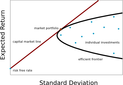
Given a quadratic utility function, it is possible to evaluate the expected utility of all linear combinations of X and Y by just knowing <X>, <Y>, <XY>, <X^2>, <Y^2>. This result generalizes to any number of investments. Using this information, for any given return, one can find the linear combination which minimizes the variance, forming the optimal portfolio for that return. The set of all optimal portfolios forms the efficient frontier in the diagram below.

Now examine the effect of adding a risk-free asset. Taking a linear combination of the risk-free asset and any given portfolio, you can achieve any new portfolio with the same Sharpe ratio (ratio of the difference between return and risk-free rate to the standard deviation) as the given portfolio. The capital market line represents the best portfolios that can be formed this way - they consist of combinations of the risk-free asset and the market portfolio, which is the efficient frontier portfolio with the largest Sharpe ratio.

Markowitz Frontier

Under the CAPM pricing model, it is assumed that stocks function as components for building market portfolios, and stockholders are only compensated for risk which cannot be diversified away by the other components. Approximating the market portfolio with the SP500, we approximate this non-diversify-able risk using the covariance between the stock and the SP500. That covariance is scaled by the variance of the market portfolio and called beta.

---

This is the standard classroom treatment of the concept of risk, and I am uncomfortable with it in ways that I will describe in the next post. For additional reading, you have wikipedia:

http://en.wikipedia.org/wiki/Modern_portfolio_theory